Business Forecasting
Operation Management
Operation Management
It would be convenient to say that ‘a lot of work has been done on forecasting and the best method is….Unfortunately, we cannot do this. Because of the wide range of things to be forecast and the different situations in which forecasts are needed, there is no single best method.
However, we can start by classifying in the different methods of forecasting, and can do this in several ways. One classification concerns the time in the future covered by forecasts. In particular;
- Long-term forecasts look ahead several years (the time typically needed to build a new factory).
- Medium-term forecasts look ahead between 3 months and two years (the time typically needed to replace an old product by a new product).
- Short-term forecasts cover the next few weeks (describing the continuing demand for a product)
The time horizon affects the choice of forecasting method because of the availability and relevance of historical data, time available to make the forecast, cost involved, effects of errors, effort considered worthwhile, and so on.
Another classification of forecasting methods draws a distinction between qualitative and quantitative approaches. For example, if a company is already making a product, it will probably have records of past demand and know the factors that affect this. Then it could use a quantitative method to forecast future demand. There are two alternatives for this;
• Projective methods, which examine the pattern of past demand and extend this into the future.
• Causal methods, which analyze the effects of outside influences and use these to produce forecasts.
Both of these approaches rely on the availability of accurate, quantified data. Suppose, though, that a company is introducing an entirely new product. There are no past demand figures that can be projected forwards, and the company does not know the factors that affect demand. In such circumstances there are no quantitative data and it must use a qualitative method. Such methods are called judgmental, and they rely on subjective assessments and opinions. However, judgmental methods use subjective assessments from various informed sources. Five widely used methods are;
• Personal insight
• Panel consensus
• Market surveys
• Historical analogy; and
• Delphi method (This is the most formal of the judgmental methods and has a well-defined procedure. A number of experts are contacted by post and each is given a questionnaire to complete).
Projective Forecasting
Projective forecasting takes historical observation and uses these to forecast future values. It ignores any external influences and only looks at past values of, say, demand to suggest future demand. Here we are going to describe 4 methods of this type;
• Simple averages
• Moving averages
• Exponential smoothing; and
• Models for seasonality and trend
These methods are most commonly used with time series, which are described as follows;
Time series:
A lot of data occur as time series, which are series of observations taken at regular intervals of time. For instance, monthly unemployment figure, daily rainfall, weekly demand, and annual population statistics.
Time Series
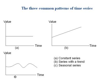
Like many other sets of data, if we have a time series the first step in analyzing it is to draw a graph, and a simple scatter diagram can show any underlying patterns. However, the 3 most common patterns in time series are;
- Constant series, in which observations take roughly the same value over time, such as annual rainfall.
- Series with a trend, which either rise or fall steadily, such as the gross national product per capita.
- Seasonal series, which have a cyclical component, such as the weekly sales of soft drinks.
These 3 patterns are shown in following slide;
If observations followed such simple patterns we would have no problems with forecasting. Unfortunately, there are nearly always differences between actual observations and the underlying pattern. A random noise is superimposed on the underlying pattern so that a constant series, for example, does not always take exactly the same value, but is some where close. So, 200, 205, 194, 195, 208, 203, 200, 193, 201, 198 is a constant series of 200 with superimposed noise.
If the noise is relatively small it is easy to get good forecasts, but if there is a lot of noise it hides the underlying pattern and forecasting becomes more difficult.
Actual value= underlying pattern +random noise
The differences between an actual observation and the value predicted by underlying pattern in a set of data is a linear trend, a graph of observations will show variations about a straight line. Each observation has an error, which is its vertical distance from the line. Then the error in period t is defined as Et.


• Exponential smoothing: Exponential smoothing is the most widely used forecasting method. It is based on the idea that as data get older they become less important and should be given less weight. In particular, exponential smoothing gives a declining weight to observations. However, a new forecast is calculated by taking a proportion, α, of the latest observation and adding a proportion,
1 – α, of the previous forecast. So,
New forecast = α x latest observation + (1 – α) x last forecast
or F t + 1= αyt + (1- α) x Ft
In this equation, α, is the smoothing constant, which usually takes a value between 0.1 and 0.2. Moreover, the given to the smoothing constant alpha (α) is important in setting the sensitivity of the forecasts. Alpha sets the balance between the last forecast and the latest observation.
--------------------------- Md Aminul Islam | maihbd@gmail.com